An Introduction to Measure Theory
With a focus on Probability

Contents

1. Introduction
2. What is a $\sigma$-algebra?
3. What is a measure?
4. Integration Theory
   1. The Lebesgue Integral
   2. Integration Theorems
5. Ergodic Theory
   1. Ergodic Theorems
6. The Big Theorems
   1. The Strong Law of Large Numbers
   2. The Central Limit Theorem
7. The Radon-Nikodym Derivative
8. Covariance Operators

Introduction

Measure theory is a branch of mathematics that generalizes the intuitive notions of length, area, and volume to more abstract settings. It provides a rigorous framework for defining and working with measures, which are functions that assign a “size” or “weight” to subsets of a given space. These measures can represent various quantities like length, area, volume, probability, or even “mass” in a generalized sense. We shall approach it with a probabilistic lens in this article.

We formally define probability distributions with a probability ensemble or triple,

\[\left( \Omega, \mathcal{F}, \mu \right).\]

In the above, $\Omega$ is the sample space: the set of all possible outcomes. $\mathcal{F}$ is the sigma-algebra ($\sigma$-algebra): a collection of subsets of $\Omega$ (events) that are “measurable”. $\mu$ is the probability measure (generalisation of a distribution). What does all of this really mean though?

What is a $\sigma$-algebra?

The $\sigma$-algebra $\mathcal{F}$ over a set $\Omega$ is a collection of subsets of $\Omega$ satisfying:

1. Contains the whole set: $\Omega \in \mathcal{F}$.
2. Closed under complement: $\mathcal{A} \in \mathcal{F} \implies \Omega \backslash \mathcal{A} \in \mathcal{F}$.
3. Closed under countable unions: $\mathcal{A}_i \in \mathcal{F} \implies \bigcup_i \mathcal{A}_i \in \mathcal{F}$.

By De Morgan’s Law, this also implies it is closed under countable intersections.

Proof De Morgan’s law states that $\bar{\mathcal{A}} \cap \bar{\mathcal{B}} = \overline{\mathcal{A} \cap \mathcal{B}}$, where we define the complement $\bar{\mathcal{A}} \equiv \Omega \backslash \mathcal{A}$.

By the closed under countable unions condition,

\[\mathcal{A}_i \in \mathcal{F} \implies \bigcup_i \mathcal{A}_i \in \mathcal{F}.\]

By the closed under complement condition,

\[\Omega \backslash \bigcup_i \mathcal{A}_i \in \mathcal{F}\]

By De Morgan’s Law,

\[\bigcap_i \left( \Omega \backslash \mathcal{A}_i \right) \in \mathcal{F}\]

Let $\mathcal{B}_i \equiv \Omega \backslash \mathcal{A}_i$, and apply the closed under complement condition,

\[\mathcal{A}_i \in \mathcal{F} \implies \mathcal{B}_i \in \mathcal{F},\\ \therefore \mathcal{B}_i \in \mathcal{F} \implies \bigcap_i \mathcal{B}_i \in \mathcal{F}.\\ \square\]

A way of gaining intuition for the $\sigma$-algebra is via a game of coin toss. Let us toss the coin twice, with $H, T$ representing heads and tails respectively. Say we only care about the number of heads (i.e. combinations rather than permutations), then our probability distribution $\left( \Omega, \mathcal{F}, \mu \right)$ is characterised as follows,

\[\Omega = \{ TT, TH, HT, HH \}, \; \mathcal{F} = \{ TT, TH, HH \}\]

and

\[\mu(X) = \begin{cases} 0.25 & X = TT \\ 0.5 & X = TH \\ 0.25 & X = HH \end{cases}, \; X \in \mathcal{F}\]

In the case where we do indeed care about permutations, we get \(\mathcal{F} = \{ TT, TH, HT, HH \}\), which is called the Borel $\sigma$-algebra, defined to be the smallest σ-algebra containing all open sets of $\Omega$.

A measurable space $(\Omega, \mathcal{F}, \mu)$ is said to be $\sigma$-finite if the whole sample space can be written as a countable union of measurable sets, each of which has finite measure, i.e.

\[\Omega = \bigcup_{i = 1}^N \mathcal{A}_i,\]

with $\mathcal{A}_i \in \mathcal{F}$ and $\mu(\mathcal{A}_i) < \infty \, \forall i$.

What is a measure?

A measure is a function that assigns a non-negative number to subsets of a set, generalizing the notion of length, are, volume, mass and probability.

Given a measurable (Borel) space $\left( \Omega, \mathcal{F} \right)$ (sample space, $\sigma$-algebra), a measure, $\mu$, is defined as

\[\mu : \Omega \rightarrow \left[0, \infty \right].\]

Take note that the infinity is bounded. This is a subtle but important point to be clarified later. The measure must satisfy the following two conditions,

1. \(\mu\left( \emptyset \right) = 0\).
2. \(\mu\left( \bigcup_i \mathcal{A}_i \right) = \sum_i \mu\left( \mathcal{A}_i \right) \;\forall \, \mathrm{disjoint} \, \mathcal{A}_i \in \mathcal{F}\).

For probability measures, there are further more stringent conditions, namely the Kolmogorov axioms, that must be satisfied.

1. \(\mu\left( \Omega \right) = 1\).
2. \(\mu\left( \Omega \right) \in \left[ 0, 1 \right]\).
3. \(\mathcal{A} \subseteq \mathcal{B} \implies \mu\left( \mathcal{A} \right) \leq \mu\left( \mathcal{B} \right)\).

Integration Theory

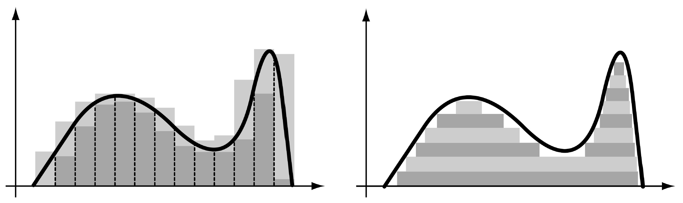Figure 1: A comparison of Riemann vs Lebesgue integration.

Two methods of integration are illustrated above, with Riemann integration on the left and Lesbegue integration on the right. Lebesgue compares the two succintly,

“I have to pay a certain sum, which I have collected in my pocket. I take the bills and coins out of my pocket and give them to the creditor in the order I find them until I have reached the total sum. This is the Riemann integral. But I can proceed differently. After I have taken all the money out of my pocket I order the bills and coins according to identical values and then I pay the several heaps one after the other to the creditor. This is my integral.”

We are used to taking the Riemann integral, since this works well with the notion of the integral being the anti-derivative. However, the Riemann integral breaks down for functions that are discontinuous almost everywhere, and does not generally permit taking limits under the integral sign. Lebesgue addresses this using the notion of simple functions and measures.

A simple function, $\varphi$, is a measurable function that takes only finitely many values, i.e.

\[\varphi = \sum_{i = 1}^n a_i \mathbb{1}_{\mathcal{A}_i}\left( x \right),\]

where $a_i \geq 0$ and \(\mathcal{A}_i \in \mathcal{F}\) are disjoint sets that span the sample space and $\mathbb{1}_{\mathcal{A}_i}(\cdot)$ is the indicator function for the set $\mathcal{A}_i$. Following this concept, we define its integral as,

\[\int_\mathcal{A} \varphi \mathrm{d} \mu = \sum_{i = 1}^n a_i \mu\left( \mathcal{A}_i \right)\]

such that ${ \mathcal{A}_i }$ are disjoint and $\bigcup_i \mathcal{A}_i = \mathcal{A}$.

N.B. Every measurable, non-negative function can be approximated by simple functions. There is a subtle point in the non-negativity that relates back to the previous bounded infinity, which we dive into next.

The Lebesgue Integral

Let $f : \Omega \rightarrow \left[0, \infty \right]$ be measurable (non-negative). We define the integral against the measure $\mu$ as follows,

\[\int_\mathcal{A} f \mathrm{d}\mu \equiv \sup\left[ \int_\mathcal{A} \varphi \mathrm{d}\mu \mid 0 \leq \varphi \leq f, \, \varphi \, \mathrm{simple} \right].\]

Referring back to the subtleties of the range: non-negativity ensures that this integral is defined, and we do not encounter an $\infty - \infty$ event. To generalise to all measurable functions, we choose $f = f^+ - f^-$ where $f^+,f^- \geq 0$. If $\int_\mathcal{A} f^+ \mathrm{d} \mu, \int_\mathcal{A} f^- \mathrm{d} \mu < \infty$, then $f$ is integrable, and we define

\[\int_\mathcal{A} f \mathrm{d} \mu = \int_\mathcal{A} f^+ \mathrm{d} \mu - \int_\mathcal{A} f^- \mathrm{d} \mu,\]

generalising to $f : \Omega \rightarrow \mathbb{R}$ and giving signed areas.

Integration Theorems

Monotone Convergence Theorem

If \(\{ f_n : n \in \mathrm{N} \}\) is a pointwise monotonically increasing sequence of positive, extended, real-valued, measurable functions, i.e.

\[f_n : \Omega \rightarrow \left[ 0, \infty \right],\] \[\cdots \leq f_n(x) \leq f_{n+1}(x) \leq \cdots \quad \forall x \in \Omega\]

and

\[f = \lim_{n \rightarrow \infty} f_n,\]

then

\[\lim_{n \rightarrow \infty} \int f_n \mathrm{d} \mu = \int f \mathrm{d} \mu.\]

The proof involves showing both $\leq$ and $\geq$ relationships between the two sides, implying equality. This is omitted.

Fatou’s Lemma

Let $\left( \Omega, \mathcal{F}, \mu \right)$ be a measure space and let \(\{ f_n \}\) be a sequence of non-negative measurable functions where $f_n : \Omega \rightarrow \left[ 0, \infty \right]$. Then the function $\lim \inf_{n \rightarrow \infty} f_n$ is measurable and

\[\int_\Omega \mathop{\liminf}_{n \rightarrow \infty} f_n \mathrm{d} \mu \leq \mathop{\liminf}_{n \rightarrow \infty} \int_\Omega f_n \mathrm{d} \mu.\]

Proof For each $n \in \mathbb{N}$, let

\[g_n := \inf _{k \geq n} f_n.\]

We know that \(\{ g_n \}\) is a monotone increasing sequence of functions, converging pointwise as

\[\lim_{n \rightarrow \infty} g_n = \mathop{\liminf}_{n \rightarrow \infty} f_n,\]

which allows for the monotone convergence theorem to apply,

\[\lim_{n \rightarrow \infty} \int_\Omega g_n \mathrm{d} \mu = \int_\Omega \mathop{\liminf}_{n \rightarrow \infty} f_n \mathrm{d} \mu.\]

Moreover, $g_n \leq f_k$ for $k \geq n$ gives

\[\begin{split} \int_\Omega g_n \mathrm{d} \mu &\leq \inf_{k \geq n} \int_\Omega f_k \mathrm{d} \mu,\\ \lim_{n \rightarrow \infty} \int_\Omega g_n \mathrm{d} \mu &\leq \mathop{\liminf}_{k \rightarrow \infty} \int_\Omega f_k \mathrm{d} \mu,\\ \int_\Omega \mathop{\liminf}_{n \rightarrow \infty} f_n \mathrm{d} \mu &\leq \mathop{\liminf}_{k \rightarrow \infty} \int_\Omega f_k \mathrm{d} \mu. \end{split}\] \[\square\]

Dominated Convergence Theorem

If \(\{ f_n \}\) is a sequence of measurable functions $f_n : \Omega \rightarrow \mathbb{R}$ such that $f_n \rightarrow f$ pointwise, and $\mid f_n \mid \leq g$ where $g : \Omega \rightarrow \left[ 0, \infty \right]$ is an integrable function, meaning $\int g \mathrm{d} \mu < \infty$, then

\[\lim_{n \rightarrow \infty} \int f_n \mathrm{d} \mu = \int f \mathrm{d} \mu.\]

Proof Since $g + f_n \geq 0$ for every $n \in \mathbb{N}$, Fatou’s Lemma implies that,

\[\int (g + f) \mathrm{d} \mu \leq \mathop{\liminf}_{n \rightarrow \infty} \int (g + f_n) \mathrm{d} \mu \leq \int g \mathrm{d} \mu + \mathop{\liminf}_{n \rightarrow \infty} \int f_n \mathrm{d} \mu.\]

By dropping $g$,

\[\int f \mathrm{d} \mu \leq \mathop{\liminf}_{n \rightarrow \infty} \int f_n \mathrm{d} \mu.\]

Similary, apply Fatou’s Lemma again, because $g - f_n \geq 0$,

\[\int (g - f) \mathrm{d} \mu \leq \mathop{\limsup}_{n \rightarrow \infty} \int (g - f_n) \mathrm{d} \mu \leq \int g \mathrm{d} \mu - \mathop{\limsup}_{n \rightarrow \infty} \int f_n \mathrm{d} \mu,\]

which gives us,

\[\int f \mathrm{d} \mu \geq \mathop{\limsup}_{n \rightarrow \infty} \int f_n \mathrm{d} \mu.\] \[\therefore \lim_{n \rightarrow \infty} \int f_n \mathrm{d} \mu = \int f \mathrm{d} \mu.\] \[\square\]

The Dominated Convergence Theorem also holds for sequences of complex-valued functions if both real and imaginary parts are measurable. Consider $f : \Omega \rightarrow \mathbb{C}$, where $f = g + \mathrm{j}h$ and $g, h \in \mathbb{R}$.

\[f \text{ is measurable} \iff g,h \text{ are measurable.} \\ f \text{ is integrable} \iff g,h \text{ are integrable.}\]

We define the integral as

\[\int f \mathrm{d} \mu = \int g \mathrm{d} \mu + \mathrm{j} \int h \mathrm{d} \mu.\]

Corollary: Bounded Convergence Theorem

Let $\mid f_n \mid \leq M$ be a uniformly bounded sequence of complex-valued, measurable functions, where $f_n \rightarrow f$ pointwise on a measurable space $\left( \Omega, \mathcal{F}, \mu \right)$ and $\mu{\Omega} < \infty$. Then $f$ is an integrable function and

\[\lim_{n \rightarrow \infty} \int f_n \mathrm{d} \mu = \int f \mathrm{d} \mu.\]

Proof $\mid f_n \mid$ is uniformly bounded by a real number $M$ for $x \in \Omega$. Define $g(x) = M \forall x \in \Omega$. $g$ is integrable since it is constant on a finitely measurable set $\Omega$. Therefore, the Dominated Convergence Theorem applies.

\[\square\]

Fubini’s Theorem

Suppose that $\left( X, \mathcal{A}, \mu \right)$ and $\left( Y, \mathcal{B}, \nu \right)$ are $\sigma$-finite measure spaces. A measurable function $f : X \times Y \rightarrow \mathbb{C}$ is integrable if and only if either of the iterated integrals

\[\int_X\left(\int_Y f \mathrm{d}\nu\right)\mathrm{d}\mu, \int_Y\left(\int_X f \mathrm{d}\mu\right)\mathrm{d}\nu\]

are finite. If $f$ is integrable, then

\[\int_{X \times Y} f (\mathrm{d} \mu \otimes \mathrm{d} \nu) = \int_X\left(\int_Y f \mathrm{d}\nu\right)\mathrm{d}\mu = \int_Y\left(\int_X f \mathrm{d}\mu\right)\mathrm{d}\nu.\]

The proof is omitted because it is long and non-trivial.

Ergodic Theory

Ergodice theory is the study of long-run behaviour. The general setting is described below:

• Measure space $(E, \mathcal{E}, \mu)$
• Measurement map $\Theta : E \rightarrow E$ which is measure preserving, i.e. $\mu(A) = \mu(\Theta^{-1}(A)), \; \forall A \in \mathcal{E}$. Note that the fact we define measure-preserving off the pre-image is significant, and this will come into play later.

Example Take $(E, \mathcal{E}, \mu) = \left(\left[0,1\right), \mathcal{B}(\left[0, 1\right)), \text{Lebesgue}\right)$. For each $a \in \left[0, 1\right)$, we can define

\[\Theta_a(x) = x+a \mod 1.\]

We know intuitively that this translation map preserves the Lebesgue measure on [0,1). The goal here is to understand long-run averages as we repeatedly apply $\Theta$.

Let $f$ be a measurable function. We define

\[S_n(f) = f + f\circ\Theta + \cdots + f\circ\Theta^{n-1},\]

where $f\circ\Theta^k$ represents the function $f$ measured from the space transformed by $\Theta$, $k$ times. We wish to know how $S_n(f)/n$ behaves as $n\rightarrow\infty$. First, let us tackle a couple definitions.

Definition Invariant Subset: We say $A\in\mathcal{E}$ is invariant for $\Theta$ if $A = \Theta^{-1}(A)$ (note the pre-image again).

Definition Invariant Function: A measurable function $f$ is invariant if $f = f\circ\Theta$.

Definition \(\mathcal{E}_\Theta\) : We write \(\mathcal{E}_\Theta = \{ A \in \mathcal{E}:A\text{ is invariant}\}\). It is easy to show \(\mathcal{E}_{\Theta}\) is a $\sigma$-algebra, and $f: E \rightarrow \mathbb{R}$ is invariant if and only if it is $\mathcal{E}_\Theta$-measurable.

Definition Ergodic: We say $\Theta$ is ergodic if $A\in\mathcal{E}_\Theta$ implies $\mu(A) = 0$ or $\mu(A^c) = 0$, where $A^c$ is the complement of $A$.

Example For the translation map $\Theta_a$ on [0,1), we have $\Theta_a$ is ergodic if and only if $a$ is irrational. To see why this is, consider that \(\mathcal{E}_{\Theta_a} = \{A\in\mathcal{E}:A = \Theta_a(A)\} = \emptyset\) if $a$ is irrational, because $\mu(B\in\mathcal{E}_\Theta) = 0$.

Proposition If $f$ is integrable and $\Theta$ is measure-preserving, then $f\circ\Theta$ is integrable and

\[\int_{\Theta(E)} f\circ\Theta\mathrm{d}\mu = \int_E f\mathrm{d}\mu.\]

Proposition If $\Theta$ is ergodic and $f$ is invariant, then there exists a constant $c$ such that $f=c$ almost everywhere, i.e. there are not many invariant functions for ergodic $\Theta$.

Example Bernoulli Shifts

Let $m$ be a probability distribution on $\mathbb{R}$. Then there exists an independent and identically distributed (i.i.d.) sequence $Y_1, Y_2,\cdots$ with law $m$. Let $E = \mathbb{R^N}$ be the set of all real sequences $(x_n)$.

Define the $\sigma$-algebra $\mathcal{E}$ to be the $\sigma$-algebra generated by the projections $X_n(x) = x_n$, i.e. it picks out the $n$-th element. In other words, this is the smalled $\sigma$-algebra such that all these functions are measurable (analogous to Borel set for $\mathbb{R}$). Alternatively, this is the $\sigma$-algebra generated by the $pi$-system

\[\mathcal{A} = \{\prod_{n\in\mathbb{N}} A_n, A_n \in \mathcal{B} \; \forall n \text{ and } A_n = \mathbb{R} \text{ eventually (for large }n\text{)}\}.\]

Finally, to define the measure $\mu$, we let $Y = (Y_1, Y_2, \cdots) : \Omega \rightarrow E$ (consider $Y(\omega) = (Y_1(\omega), Y_2(\omega), \cdots)$ where $\omega \in \Omega$), where $Y_i$ are the i.i.d. random variables defined above and $\Omega$ the sample space of $Y_i$. Then, $Y$ is a measurable map because each of the $Y_i$’s is a random variable. $\mu$ measures the likelihood of an infinite sequence landing in a given set $A$. Let $\mu = \mathbb{P} \circ Y^{-1}$

\[\implies \mu(A) := \mathbb{P}(Y^{-1}(A)) \; \forall \text{ measurable } A \subseteq \mathbb{R^N}.\]

By independence, we see that

\[\mu(A) = \prod_{n \in \mathbb{N}} m(A_n),\]

for any cylinder set $A = A_1 \times A_2 \times \cdots \times A_n \times \mathbb{R} \times \cdots \times \mathbb{R}$, i.e. the first $n$ elements (degrees of freedom) are constrained, the rest are unconstrained. Note that this product $\mu$ is eventually 1, so is finite.

$(E, \mathcal{E}, \mu)$ as defined above is the canonical space associated with the sequence of i.i.d. random variables with law $m$.

Define $\Theta : E \rightarrow E$ by

\[\Theta (x) = \Theta (x_1, x_2, x_3, \cdots) = (x_2, x_3, \cdots).\]

This is the shift map. This is useful in conjunction with the function,

\[f(x) = f(x_1, x_2, \cdots) = x_1,\] \[\implies S_n(f) = f + f\circ\Theta + \cdots + f\circ\Theta^{n-1} = x_1 + \cdots + x_n,\]

i.e. the $n$-sum of elements in the sequence.

Theorem The shift map $\Theta$ is an ergodic, measure-preserving transformation.

Proof Use the tail $\sigma$-algebra, defined as

\[\mathcal{T}_n = \sigma(X_m : m\geq n+1) \implies \mathcal{T} = \bigcup_n \mathcal{T}_n.\]

This $\sigma$-algebra is insensitive to changes in any finite number of elements. Suppose that $A \in \prod_{n \in \mathbb{N}} A_n \in \mathcal{A}$. Then,

\[\Theta^{-n} = \{X_{n+k} \in A_k \; \forall k\} \in \mathcal{T}_n.\]

Since $\mathcal{T}_n$ is a $\sigma$-algebra, and $\Theta^{-n}(A)\in\mathcal{T}_n\; \forall A \in \mathcal{A}$ and $\sigma(\mathcal{A}) = \mathcal{E}$, we know $\Theta^{-n}(A)\in\mathcal{T}_n \;\forall A \in \mathcal{E}$.

So if $A \in \mathcal{E}_\Theta$, i.e. $A = \Theta^{-1}(A)$, then $A\in\mathcal{T}_n\;\forall n$.

\[A \in \mathcal{T}.\]

From the Kolmogorov 0-1 Law, which states that all tail events have either a 0 or 1 probability, we know etiher

\[\mu(A) = 0 \text{ or } 1\] \[\therefore \Theta \text{ is ergodic}.\]

Next, we must show $\Theta$ to be measurable and measure-preserving. Consider the $\pi$-system above,

\[\begin{split} \mathcal{A} &= \{\prod_{n\in\mathbb{N}} A_n, A_n \in \mathcal{B} \; \forall n \text{ and } A_n = \mathbb{R} \text{ eventually (for large }n\text{)}\}\\ &\equiv A_1 \times A_2 \times \cdots \times A_n \times \mathbb{R} \times \cdots \times \mathbb{R}. \end{split}\] \[\mu(\mathcal{A}) = \prod_{i=1}^n \mu(A_i)\]

To show $\Theta$ is measure-preserving for the above, we must show

\[\mu(\mathcal{A}) = \mu(\Theta^{-1}(\mathcal{A})).\]

We know the pre-image is the set of all things that map onto $\mathcal{A}$ and in this case is defined as,

\[\Theta^{-1}(\mathcal{A}) = \mathbb{R} \times A_1 \times A_2 \times \cdots \times A_n \times \mathbb{R} \times \mathbb{R} \times \cdots.\] \[\mu(\Theta^{-1}(\mathcal{A})) = \mu(\mathcal{A})\]

trivially because $\mu(\mathbb{R}) = 1$.

\[\square\]

Ergodic Theorems

Proofs have not been included.

Maximal Ergodic Lemma

Let $f$ be integrable, and

\[S^* = \sup_{n\geq 0} S_n(f) \geq 0,\]

where $S_0(f) = 0$ by convention. Then,

\[\int_{\{S*>0\}} f \mathrm{d}\mu \geq 0.\]

Birkhoff’s Ergodic Theorem

Let $(E, \mathcal{E}, \mu)$ be $\sigma$-finite and $f$ be integrable. There exists an invariant function $\bar{f}$ such that

\[\mu(\mid \bar{f} \mid) \leq \mu( \mid f \mid) \text{ and } S_n(f)/n \rightarrow \bar{f} \text{ a.e.}\]

If $\Theta$ is ergodic, then $\bar{f}$ is constant (from above). Note that this theorem gives an inequality, but in many cases we can apply integration theorems to argue equality.

Von Neumann’s Ergodic Theorem

Let $(E, \mathcal{E}, \mu)$ be a finite measure space. Let $p\in[1,\infty)$ and assume that $f \in \mathcal{L}^p$. Then, there is some function $f\in\mathcal{L}^p$ such that

\[\frac{S_n(f)}n \rightarrow \bar{f} \in \mathcal{L}^p.\]

The Big Theorems

Next, we dive into the two most important theorems about the sums of independent random variables.

The Strong Law of Large Numbers

The Strong Law of Large Numbers Assuming Finite 4^th Moments

Let $(X_n)$ be a sequence of independent random variables such that there exists $\mu \in \mathbb{R}$ and $M>0$ such that

\[\mathbb{E}\left[X_n\right] = \mu,\; \mathbb{E}\left[X_n^4\right] \leq M \; \forall n.\]

With $S_n = X_1 + \cdots + X_n$, we have

\[\lim_{n\rightarrow \infty}\frac{S_n}{n} \rightarrow \mu \text{ a.s.}\]

Note that we do not require that $X_n$ be i.i.d. here, only independent and the same mean. We cast the constraint onto the finite 4^th moments condition. a.s. stands for almost surely, i.e. the event fails only on a set of probability zero. This is a funny notion, but you can imagine it being similar to the idea of $\mathbb{P}(X = a) = 0, \; \forall a \in \Omega$ for any continuous distribution.

Proof We reduce the problem to the case where $\mu = 0$ by defining

\[Y_n = X_n - \mu.\]

We then have

\[\begin{split} \mathbb{E}\left[Y_n\right] = 0, \;\mathbb{E}\left[Y_n^4\right] &\leq 2^4 \left(\mathbb{E}\left[\mu^4 + X_n^4\right]\right)\\ \mathbb{E}\left[Y_n^4\right] &\leq 2^4 \left(\mu^4 + M\right). \end{split}\]

Therefore, it suffices to show the theorem holds for $Y_n$ in place of $X_n$. Hence, in the following $\mathbb{E}\left[X_n\right] = 0$.

By independence, we know that for $i \neq j$,

\[\mathbb{E}\left[X_i X_j^3\right] = \mathbb{E}\left[X_i\right] \mathbb{E}\left[X_j^3\right] = 0.\]

Similarly, for distinct $i, j, k, l$,

\[\mathbb{E}\left[X_i X_j X_k^2\right] = \mathbb{E}\left[X_i X_j X_k X_l\right] = 0.\]

Hence, we know that by polynomial expansion,

\[\mathbb{E}\left[S_n^4\right] = \mathbb{E}\left[\sum_{k=1}^n X_k^4 + 6\sum_{1 \leq i < j \leq n} X_i^2 X_j^2\right].\]

The first term is bounded by $nM$ by linearity, and we know for $i\neq j$,

\[\mathbb{E}\left[X_i^2 X_j^2\right] = \mathbb{E}\left[X_i^2\right] \mathbb{E}\left[X_j^2\right] \leq \sqrt{\mathbb{E}\left[X_i^4\right] \mathbb{E}\left[X_j^4\right]} \leq M\]

by Jensen’s inequality (consider the two terms separately and that $\sqrt{\cdot}$ is concave). By considering combinations and triangle numbers, we get

\[\mathbb{E}\left[6\sum_{1 \leq i < j \leq n} X_i^2 X_j^2\right] \leq 3n(n-1)M.\]

Putting everything together, we have

\[\mathbb{E}\left[S_n^4\right] \leq nM + 3n(n-1)M \leq 3n^2M\] \[\begin{split} \mathbb{E}\left[\left(\frac{S_n}{n}\right)^4\right] &\leq \frac{3M}{n^2}\\ \mathbb{E}\left[\sum_{n = 1}^\infty\left(\frac{S_n}{n}\right)^4\right] &\leq \sum_{n = 1}^\infty\frac{3M}{n^2} < \infty\\ \sum_{n = 1}^\infty\left(\frac{S_n}{n}\right)^4 &< \infty \text{ a.s.}\\ \text{i.e.} \frac{S_n}{n} &\rightarrow 0 \text{ a.s.}\\ \end{split}\] \[\square\]

Next we tackle the SLLN without the assumption of finite fourth moments, instead requiring i.i.d. random variables.

The Strong Law of Large Numbers

Let $(Y_n)$ be an i.i.d. sequence of integrable random variables with mean $\nu$. WIth $S_n = Y_1 + \cdots + Y_n$, we have

\[\frac{S_n}{n} \rightarrow \nu \text{ a.s.}\]

Proof The following proof requires ergodic theory (see above) but is elegant.

Let $m$ be the law of $Y_1$ and let $Y = (Y_1, Y_2, Y_3, \cdots)$. We can view $Y$ as a function

\[Y : \Omega \rightarrow \mathbb{R^N} = E.\]

Let $(E, \mathcal{E}, \mu)$ be the canonical space associated with the distribution $m$, so that

\[\mu = \mathbb{P} \circ Y^{-1}.\]

We let $f : E \rightarrow \mathbb{R}$ be given by

\[f(x_1, x_2, \cdots) = X_1(x_1, x_2, \cdots) = x_1.\]

Then $X_1$ has law given by $m$, and in particular is integrable. Also, the shift map $\Theta : E \rightarrow E$, which is given by

\[\Theta(x_1, x_2, x_3, \cdots) = (x_2, x_3, \cdots),\]

is measure-preserving and ergodic.

Thus, with

\[\begin{split} S_n(f) &= f + f\circ\Theta + \cdots + f\circ\Theta^{n-1}\\ &= X_1 + X_2 + \cdots + X_n, \end{split}\]

we have that $\frac{S_n(f)}{n} \rightarrow \bar{f} \text{ a.e.}$ by Birkhoff’s Ergodic Theorem.

We also have convergence in $\mathcal{L}^1$ by von Neumann’s Ergodic Theorem. Here, $\bar{f}$ is $\mathcal{E}_\Theta$-measurable, and $\Theta$ is ergodic, so we know that $\bar{f} = c$ almost everywhere for some constant $c$. Moreover,

\[\begin{split} c = \mu(\bar{f}) &= \lim_{n \rightarrow \infty} \mu(\frac{S_n(f)}{n})\\ &= \nu \end{split}\] \[\square\]

The Central Limit Theorem

Let \(\{ X_n \}\) be a sequence of i.i.d. random variables with $\mathbb{E}\left[X_i\right] = 0$ and $\mathbb{E}\left[X_i^2\right] = 1$. Then, if we set

\[S_n = X_1 + \cdots + X_n,\]

we have

\[\lim_{n\rightarrow\infty} \mathbb{P}\left[ \frac{S_n}{\sqrt{n}} \leq x \right] \rightarrow \int_{-\infty}^x \frac{e^{-y^2/2}}{\sqrt{2\pi}}\mathrm{d} y = \mathbb{P}\left[Z \leq x\right], \; \forall x \in \mathbb{R},\]

where $Z \sim N \left(0,1\right)$ is the standard normal variable.

Proof Let $\varphi(u) = \mathbb{E}\left[e^{\mathrm{j}uX_1}\right]$. Since $\mathbb{E}\left[X_1^2\right] = 1 < \infty$, we can differentiate under the expectation twice to obtain

\[\begin{split} \varphi'(u) &= \mathbb{E}\left[\mathrm{j}X_1e^{\mathrm{j}uX_1}\right],\\ \varphi''(u) &= \mathbb{E}\left[-X_1^2e^{\mathrm{j}uX_1}\right]. \end{split}\]

Note that we use complex moment generating functions to ensure boundness, since $\mid e^{\mathrm{j}\theta} \mid = 1 < \infty$.

Evaluating at 0, we have

\[\begin{split} \varphi(0) & = 1,\\ \varphi'(0) & = 0,\\ \varphi''(0) & = -1. \end{split}\]

So Tayler expanding $\varphi$ around 0, we have

\[\varphi(u) = 1 - \frac{u^2}{2} + \mathcal{O}(u^2).\]

We consider the generating function of $S_n/\sqrt{n}$,

\[\begin{split} \varphi_n(u) &= \mathbb{E}\left[e^{\mathrm{j}uS_n/\sqrt{n}}\right]\\ &= \prod_{i = 1}^n \mathbb{E}\left[e^{\mathrm{j}uX_i/\sqrt{n}}\right]\\ &= \varphi(u/\sqrt{n})^n\\ &= \left(1 - \frac{u^2}{2n} + \mathcal{o}\left(\frac{u^2}{n}\right)\right)^n. \end{split}\]

Taking the logarithm,

\[\begin{split} \log \varphi_n(n) &= n \log \left( 1 - \frac{u^2}{2n} + \mathcal{o}\left(\frac{u^2}{n}\right) \right)\\ &= -\frac{u^2}2 + \mathcal{o}(1) \rightarrow -\frac{u^2}2. \end{split}\] \[\therefore \varphi_n(u) \rightarrow e^{-\frac{u^2}2}.\]

which is the generating function of an $N(0,1)$ random variable. So, we have convergence in generating function. Hence, weak convergence and convergence in distribution.

\[\square\]

The Radon-Nikodym Derivative

Let $(\Omega, \mathcal{F})$ be a measurable space, where

• $\mu$ is a $\sigma$-finite measure on $(\Omega, \mathcal{F})$
• $\nu$ is another $\sigma$-finite measure on the same space. We say $\nu \ll \mu$ ($\nu$ is absolutely continuous w.r.t. $\mu$) if

\[\mu(\mathcal{A}) = 0 \implies \nu(\mathcal{A}) = 0, \;\forall \mathcal{A} \in \mathcal{F}.\]

Radon-Nikodym Theorem

Suppose $\nu \ll \mu$ and $\mu$ is $\sigma$-finite. Then there exists a measurable function $f : \Omega \rightarrow \left[ 0, \infty \right] \text{ s.t. } \forall \mathcal{A} \in \mathcal{F}$,

\[\nu(\mathcal{A}) = \int_\mathcal{A} f \mathrm{d} \mu.\]

Moreover, this function $f$ is unique up to $\mu$-almost-everywhere equality, and it is called the Radon Nikodym derivative of $\nu$ w.r.t. $\mu$ denoted $f = \mathrm{d}\nu / \mathrm{d}\mu$.

To clarify, the $\mu$-almost-everywhere equality means,

\[\mu(A \triangle B) = 0,\]

where we define $A \triangle B := (A \cap \bar{B}) \cup (\bar{A} \cap B)$, i.e.

\[\nu(\mathcal{A}) = \nu(\mathcal{B}) \iff \mu(\mathcal{A} \triangle \mathcal{B}) = 0.\]

In probability, this is the condition where the symmetric difference set has no chance of occurring, so can be intuitively ignored ($\mathcal{A}$ and $\mathcal{B}$ would be functionally identical).

The Radon-Nikodym derivative can be used in conjuntion with Baye’s Theorem,

\[f = \frac{\mathrm{d}\nu}{\mathrm{d}\mu} \implies f = \frac{p(\mathcal{A}\mid\mathcal{D})}{p(\mathcal{A})},\]

where $p(\cdot)$ is a probability density function (pdf). In this case, the Radon-Nikodym derivative represents the change in pdfs with influx of data and information (the ratio of Posterior to Prior distributions).

Covariance Operators

Consider, for $x, y \in \mathbb{R}^n$, we get a covariance matrix

\[\mathbb{Cov}(x,y) \in \mathbb{R}^{n\times n}.\]

A matrix is a bilinear form. That is to say, it is an operator that can act on 2 vectors in a bilinear (linear on one at a time) fashion, e.g.

\[\langle a, b \rangle _\mathbb{Cov} = a^T \left[\mathbb{Cov}\right]b, \; \forall a,b \in \mathbb{R}^n.\]

Generally, we can write this bilinear form as an operator

\[\mathcal{C}(a,b):=a^T \left[\mathbb{Cov}\right]b.\]

In this section, we find a way to generalise this to infinite dimensions. Also, note that I have not used bold font, order any other markers for vectors, for sake of generality.

First, let is gather some intuition for infinite dimensions. $\mathbb{R}^\infty$ can be perceived as a function space, with each element in the vector defining the function pointwise, e.g. $\mathcal{L}^p$, which is the set of $p$-integrable functions. In this isomorphism, discrete $\mathbb{R}^n$ vectors can be perceived as representing finite samples of functions. Note that countable and uncountable infinities will simply be accounted for by the function input parameter space $\Omega$. For Hilbert function spaces, the inner product is defined,

\[\langle x, y \rangle = \int_\Omega x(t)y(t)\mathrm{d}t, \; \forall x,y\in\mathcal{L}^p,\]

where functions in $\mathcal{L}^p$ act upon the parameter space $\Omega$. Consider

\[\mathbb{E}\left[ \langle x, Z \rangle \langle y, Z \rangle \right],\]

where $x$ and $y$ are fixed (input) vectors and $Z$ is a random variable of zero-mean.

\[\begin{split} \mathbb{E}\left[ \langle x, Z \rangle \langle y, Z \rangle \right] &= \mathbb{E}\left[\int_\Omega x(t)Z(t)\mathrm{d}t\int_\Omega y(\tau)Z(\tau)\mathrm{d}\tau\right]\\ &=\mathbb{E}\left[\int_\Omega x(t)\{\int_\Omega Z(t)Z(\tau)y(\tau)\mathrm{d}\tau\}\mathrm{d}t\right]\\ &=\int_\Omega x(t)\{\int_\Omega \mathbb{E}\left[Z(t)Z(\tau)\right]y(\tau)\mathrm{d}\tau\}\mathrm{d}t. \end{split}\]

Now observe that $Z(t)Z(\tau)$ is the function tensor product of $Z(t)$ and $Z(\tau)$ and

\[\mathbb{E}\left[Z(t)Z(\tau)\right] = \mathbb{Cov}\left(Z(t), Z(\tau)\right) + \mathbb{E}\left[Z(t)\right]\mathbb{E}\left[Z(\tau)\right].\]

We should note here that $Z \sim (\mathcal{L}^p, \mathcal{F}, \mu)$.

\[\mathbb{E}\left[Z(t)\right] := \mathbb{E}_\mu\left[Z(t)\right]\]

is independent of parameterization, and since $Z$ is zero-mean,

\[\implies \mathbb{E}\left[Z(\cdot)\right] = 0.\] \[\therefore \mathbb{E}\left[Z(t)Z(\tau)\right] = \mathbb{Cov}\left(Z(t), Z(\tau)\right).\]

Note that the tensor product tells us that this is a bilinear form. Let us denote this covariance in its operator form, i.e.

\[\mathbb{Cov} \left(Z(t), Z(\tau)\right) = \mathcal{C}(t,\tau),\] \[\mathbb{E}\left[ \langle x, Z \rangle \langle y, Z \rangle \right] = \int_\Omega x(t)\{\int_\Omega \mathcal{C}(t, \tau)y(\tau)\mathrm{d}\tau\}\mathrm{d}t.\]

Let $\mathcal{C}(t,\tau) = \mathcal{C}^t(\tau)$, i.e. the linear operator parameterised by $t$ acting on $\tau$.

\[\begin{split} \mathbb{E}\left[ \langle x, Z \rangle \langle y, Z \rangle \right] &= \int_\Omega x(t)\{\int_\Omega \mathcal{C}^t(\tau)y(\tau)\mathrm{d}\tau\}\mathrm{d}t\\ &= \int_\Omega x(t) \langle \mathcal{C}^t, y \rangle \mathrm{d}t\\ &= \int_\Omega x(t) \left[ \mathcal{C}y \right](t) \mathrm{d}t\\ &= \langle x, \mathcal{C}y \rangle \end{split}\]

Note that by symmetry, and the definition of an adjoint operator (shown below),

\[\langle \mathcal{C}^*x, y \rangle = \langle x, \mathcal{C}y \rangle,\]

$\mathcal{C}$ is self-adjoint. Therefore, $\mathcal{C} : \mathcal{L}^p \rightarrow \mathcal{L}^p$ and behaves in the same manner as its finite counterpart,

\[\begin{split} \mathcal{C} y &\iff \mathbb{Cov} y,\\ \langle x, \mathcal{C} y \rangle &\iff x^T \mathbb{Cov} y. \end{split}\]

As a corollary, $\mathbb{E}\left[ \langle x, Z \rangle \langle x, Z \rangle \right] = \langle x, \mathcal{C} x \rangle$,

\[\langle x, \mathcal{C} x \rangle = \mathbb{E}\left[ \langle x, Z \rangle ^2 \right] \geq 0.\]

Therefore $\mathcal{C}$ is positive semi-definite.

19/08/2025