Segmenting MRI Density/Magnitude Scans with a Fully Convolutional Network (FCN) ResNet

This project can be found on my GitHub.

This sub-project explores segmenting MRI scans with Fully Convolutional Networks. The application of this particular segmentation is to use the segmentation as a high quality first estimate for blood vessel boundaries, which will then be refined using an iterative solver. The refined boundaries will then be used as a prior for the Inverse Navier-Stokes Problem. See Prof Matthew Juniper’s website for more details on the full project.

The FCN ResNet and U-Net Architectures

A Fully Convolutional Network (FCN) is effectively a Convolutional Neural Network (CNN) without a fully connected layer at its output. In other words, whereas a CNN takes an image in and spits out an output which is different in shape (e.g. a vector of class logits or a single binary class), an FCN outputs something of the same shape as the input (e.g. N $\times$ H $\times$ W tensor for an N-channel H $\times$ W image input).

The term ResNet is an abbreviation of Residual Network. Simply speaking, a ResNet uses residual blocks, which employ skip connections to combine the input with the output of the block. This addresses the vanishing gradients problem (where backpropagated gradients become very small). Residual blocks and skip connections allow a ResNet to have very deep networks with many layers, e.g. the ResNets used in this project had 50 and 101 layers.

The U-Net (Ronneberger et al., 2015) is an FCN designed for Biomedical Image Segmentation. The U-Net generalises well between 2D and 3D, since all the convolutional and deconvolutional layers can be easily interchanged. Additionally, the U-Net learns to account for both low-level and high-level features in segmentation, due to the skip connections, which also leads to greater training stability.

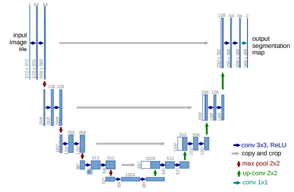Figure 1: The U-Net Architecture

Loss Function and Training Scheme

With regards to the loss functions, I tested the Weighted Cross-Entropy, DICE and Focal-Tversky Losses, as well as combinations.These choices of loss functions allow us to preferentially target accurate positive (foreground) prediction, since the training data tends to sparse (majority background). The combinations seemed to lead to training instability and exploding gradients. After comparing the three, it was deemed that the Focal-Tversky loss performed best, with the fastest convergence and best Validation IoU scores.

The training scheme employs two-level patience, with a patience-base learning rate scheduler (reduces LR on plateau) and patience-based early stopping in training to prevent overfiting. Combined with an AdamW regularised optimiser, which employs weight decay for L2 regularisation, this leads to very good generalisation and performance.

Data

One of the largest difficulties of this project is the lack of quality pre-segmented data. To overcome this, we use a level set method to generate artificial data. The process is described below:

1. Use analytical methods or pre-written packages to generate a seed SDF. In this repo, I have written classes for tubes and circles. New seed geometries can be used by parsing the new SDF into the utils.data_gen_utils.SDF_MRI base class initialization.
2. Generate a speed field and modulate it with random functions.
3. Apply the speed field to the seed SDFs to perturb the geometry, forming a new SDF.
4. Apply an activation to the SDF with noise for the magnitude replica.
5. Apply a np.where() method for the binary mask.

In step 4, we add a combination of Gaussian white noise and correlated noise (sampled from an untrained Gaussian Process), to give accurate-looking MRI data.

We reserve real segmented MRI data for the validation set.

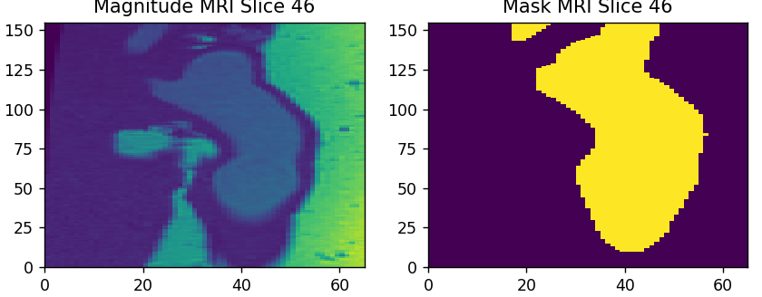Figure 2: This is a slice of the Aorta density scan.

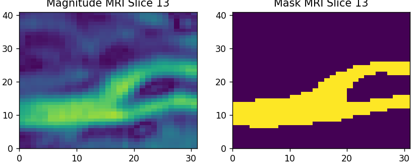Figure 3: This is a slice of the Carotid density scan.

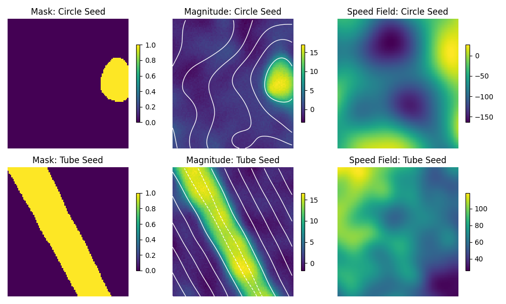Figure 4: This is a slice of the artificially generated density scan. The white lines overlayed on the magnitude scan are Signed Distance Field contours.

Note: The real MRI data is not yet publicly available.

Results

Figure 5. Initial (only real data and warped real data) performance on Aorta Coarctation.

Figure 6: Performance on Aorta after training on artificial data.

(a) Aorta Coarctation (b) Aorta (c) Carotid Figure 7: Performance after hyperparameter fine-tuning, model and loss selection & data-split tuning.

Next Steps

Running the repo

Clone the repo, then run

pip install requirements.txt

and the install torch from the official PyTorch website.

The data folder should be formatted as:

data/
├── train/
|   ├── magn/
|   |   ├──train_file_name_1
|   |   ├──train_file_name_2
|   |   :
|   └── mask/
|       ├──train_file_name_1
|       ├──train_file_name_2
|       :
└── val/
    ├── magn/
    |   ├──val_file_name_1
    |   ├──val_file_name_2
    |   :
    └── mask/
        ├──val_file_name_1
        ├──val_file_name_2
        :

27/08/2025